Denoise First, Orthogonalize Later: Understanding Momentum in Muon via Spectral Filtering

Sign up for free to create and run prompts on this paper using GPT-5.

What this paper is about (big picture)

This paper studies a training method for neural networks called Muon. Muon makes updates using matrices (tables of numbers) instead of treating each number separately. In practice, Muon works best when you first smooth the gradients with momentum and then “orthogonalize” them (a special kind of straightening). The paper explains why this order matters: momentum acts like a smart noise filter, so “denoise first, then orthogonalize” gives better, more stable updates.

The main questions the paper asks

• Why does adding momentum inside Muon help so much in training large models like LLMs?
• Does the order of steps matter? Is it better to: 1) smooth with momentum first and then orthogonalize (the Muon way), or 2) orthogonalize each step first and then average with momentum, or 3) skip momentum and only orthogonalize?
• What exactly is momentum doing to the gradient information that makes the final update more accurate?

How they studied it (simple explanation of the approach)

Think of each training step’s gradient as a song mixed with static:

• “Signal” = the part we actually want (the song).
• “Noise/perturbation” = random junk added on top (the static).

The paper uses a common model: each gradient = signal + noise. They assume:

• The important directions of the signal don’t jump around wildly over short periods (the song keeps the same melody).
• The noise averages out over time (it’s random and doesn’t line up consistently).

Momentum is like a running average:

• It combines recent gradients using a rule: $M_t = \beta M_{t-1} + (1-\beta) G_t$ Here $G_t$ is the current gradient, and $M_t$ is the smoothed version. A larger $\beta$ (close to 1) means “remember more of the past,” which smooths more strongly.
• The “effective window” of smoothing is $T = \frac{1}{1-\beta}$. Bigger $T$ means more smoothing.

Orthogonalization (Muon's special step) is like straightening the directions while ignoring how big they are. In math, this is called taking a “polar factor”: it keeps the direction information of the gradient matrix but resets all the sizes (amplitudes) to 1.

The key idea:

• If you orthogonalize too early, you erase the helpful size differences that tell signal apart from noise.
• If you smooth first, momentum lowers the noise and keeps the important directions, so the later orthogonalization works on a cleaner, more reliable matrix.

They back this up with:

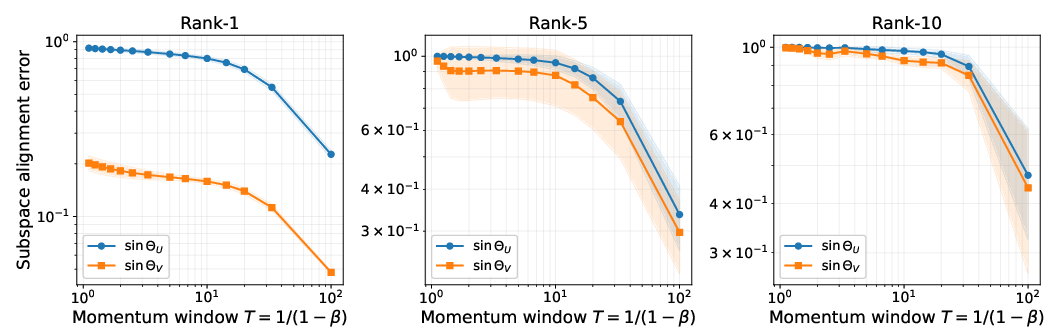
• Math proofs that momentum creates a bigger gap between strong “signal directions” and weaker “noise directions.” This is called enlarging the “spectral gap,” which means the important directions stand out clearly.
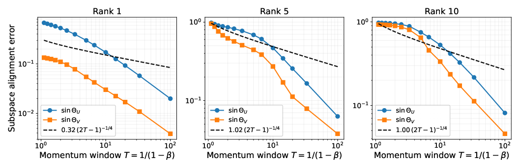
• Proofs that when that gap is bigger, the directions you extract (the “top subspaces”) line up better with the true signal.
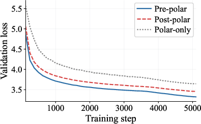
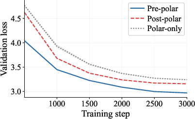
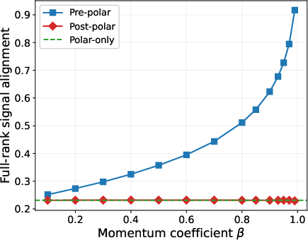
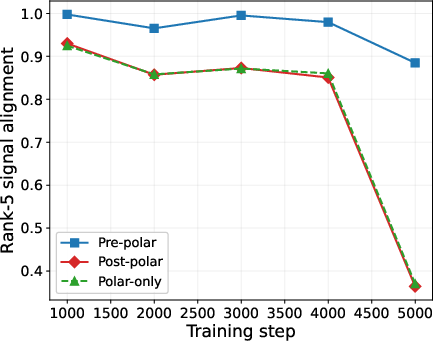
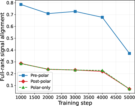
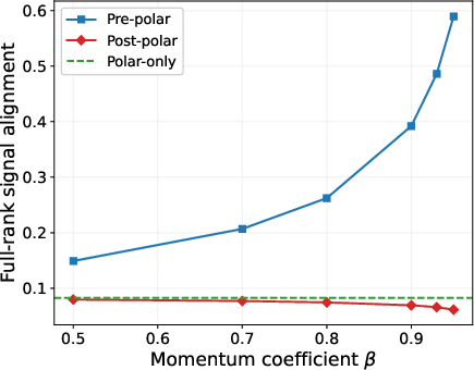
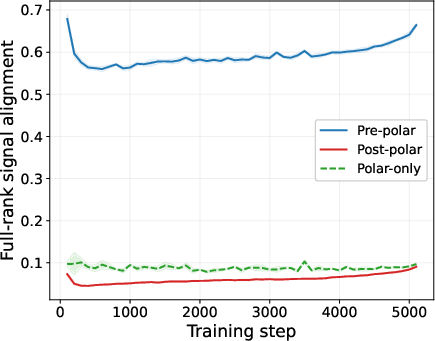
• Head-to-head comparisons of three pipelines: 1) Pre-polar (momentum first, then orthogonalize), 2) Post-polar (orthogonalize each step first, then momentum), 3) Polar-only (orthogonalize without momentum).
• Experiments on real training (like NanoGPT and LLaMA 350M) and controlled tests that collect many gradients and analyze them.

What they found and why it matters

Here are the main results in everyday terms:

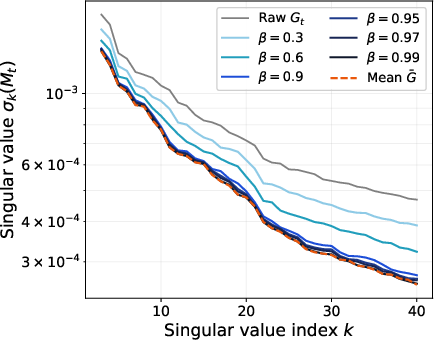
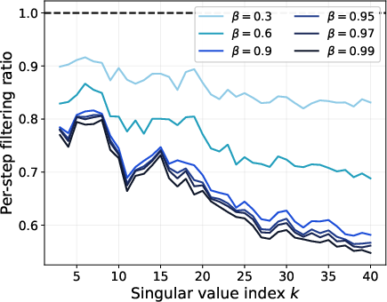
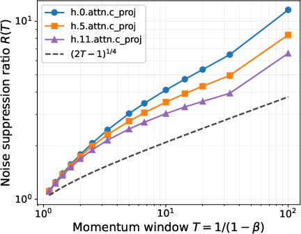
• Momentum is a spectral filter. In music terms: it lowers the volume of random static while keeping the melody strong. Mathematically, after momentum, the strongest directions (signal) stay strong, and the weak, noisy directions get quieter. This creates a clear gap that helps us tell signal from noise.
• The order of operations is critical.
  • Pre-polar (momentum → orthogonalize) works best because the orthogonalization step sees a clean, denoised matrix and can lock onto the right directions.
  • Post-polar (orthogonalize → momentum) performs worse. Once you orthogonalize early, you erase the size differences that help separate signal from noise; averaging afterward can’t bring that information back.
  • Polar-only (orthogonalize with no momentum) is the most fragile, especially when the true signal is faint compared to noise; the paper shows cases where it basically fails to find the signal as matrices get larger.
• Bigger momentum (β closer to 1) helps more. With a larger effective window $T$, noise is suppressed more strongly, the “spectral gap” gets larger, and the directions become more reliable.
• Real experiments confirm the theory. On tasks like NanoGPT and LLaMA 350M training, the Pre-polar pipeline consistently outperforms the other two. The data shows exactly what the math predicts: smoothing first makes the directions cleaner, and learning proceeds faster and more reliably.

Why this matters: It explains a real mystery—why Muon works so well with momentum—and gives a simple, powerful design rule for optimizers that use matrix operations on gradients.

What this means going forward

• A clear design rule: denoise first, then orthogonalize. If your optimizer uses a nonlinear “direction-only” step (like Muon’s orthogonalization), you should first apply a good filter (momentum) that separates signal from noise. Doing things in the wrong order can permanently lose useful information.
• Better optimizer design for big models. Understanding momentum as a spectral filter—not just a speed-up trick—helps us tune it wisely and consider new variants that might filter even better.
• Limits and next steps:
  • The paper focuses on a common momentum form; popular variations like Nesterov momentum weren’t fully analyzed here.
  • It proves a strong separation in a clean, rank-1 “spiked” model and shows broad evidence in practice, but sharper proofs for more complex signals and different noise types remain future work.
  • Schedules that change momentum over time (common in practice) are promising but need more theory.

In short: The paper shows that Muon’s success comes from using momentum as a noise filter before orthogonalizing. This simple idea—denoise first, then straighten—makes updates more stable and aligned with what the network truly needs to learn.

Knowledge gaps, limitations, and open questions

Below is a concise list of what remains missing, uncertain, or unexplored in the paper, written to guide concrete future work:

• Theory assumes a structured gradient model with temporally coherent, time-invariant singular directions; extending results to dynamically rotating/ drifting signal subspaces (nonstationary or slowly varying $U,V$) is open.
• The “signal persistence” assumption introduces an unknown constant $c_{\mathrm{sig}}$ and assumes $|\bar\lambda_k(t)|\ge c_{\mathrm{sig}}\lambda_k$; there is no procedure to verify or estimate $c_{\mathrm{sig}}$ from data or to characterize failure modes when it is small.
• Noise model requires bounded variance, mean-zero, and inter-step orthogonality (and sometimes pairwise independence) of perturbations; real gradient noise is often autocorrelated and heavy-tailed—extensions to temporally correlated, biased, or infinite-variance noise are not developed.
• Main separation theorem (Pre-polar > Post-polar/Polar-only) additionally assumes a time-invariant signal and absolutely continuous perturbations; robustness to departures from these (e.g., discrete or mixture noise distributions) is not analyzed.
• Quantitative separation is only proven for the rank-1 spiked Gaussian model in a low-SNR regime; generalizing to rank-$r$ signals, anisotropic/structured noise, and moderate/high SNR remains open.
• The spectral-gap and subspace-reliability rates scale as $(2T-1)^{-1/4}$; it is unclear whether these rates are tight or can be improved (e.g., to $(2T-1)^{-1/2}$) under stronger or alternative assumptions.
• Analysis focuses on constant-$\beta$ EMA/Polyak momentum; time-varying momentum schedules (commonly used in practice) and their effect on filtering and ordering are not theoretically treated.
• Nesterov momentum (often used with Muon) is out of scope; the paper does not analyze how the extra “lookahead” term alters the spectral filtering and ordering conclusions.
• The polar factor is treated as exact; practical Muon uses Newton–Schulz iterations with approximation error. How approximation error composes with momentum filtering, and whether error interacts with $T$ or spectrum shape, is not analyzed.
• Only the order “denoise (momentum) → orthogonalize (polar)” and its reversal are compared; alternatives (e.g., partial/soft orthogonalization, spectral shrinkage before/after polar, mixed or iterative ordering) are not explored.
• Theoretical results assume $m\ge n$; behavior for $m<n$, very rectangular matrices, or block/tensor-structured parameters (e.g., convolutions) is not characterized.
• The link from improved signal alignment to concrete optimization guarantees (loss decrease, convergence rate, sample efficiency) and generalization outcomes is not established.
• Trade-offs under nonstationarity are not quantified: how large $T$ can be before momentum lag harms tracking when signal subspaces evolve over training.
• Optimal filter design is not studied: whether other (FIR/IIR) kernels, windowed averages, multi-tap or frequency-selective filters could achieve larger spectral gaps or better tracking than EMA.
• Interaction with adaptive methods (e.g., AdamW’s per-parameter scaling) is not analyzed; whether “denoise → orthogonalize” still dominates when combined with adaptive scaling remains unknown.
• No guidance for choosing $T$ (or $\beta$) relative to dimension, SNR, or noise statistics; explicit formulas or bounds for the minimal $T_0$ in Theorem 2 are not provided.
• The empirical probes (stationary and trajectory) rely on the in-buffer mean $\bar G$ as a proxy for the true signal; bias and variance of this proxy under drifting signals, and its effect on measured alignment, are not quantified.
• Sensitivity to other training hyperparameters (learning rate, batch size, clipping, weight decay, warmup/warmdown schedules) and their interaction with momentum filtering is not systematically evaluated.
• Robustness to practical implementation details (e.g., low-precision arithmetic, randomized or truncated SVD, number of Newton–Schulz iterations) is not assessed.
• Distributed/large-scale training settings (communication/computation effects of polar/EMA order, asynchrony, and staleness) are not explored.
• Empirical scope is limited relative to the breadth of modern architectures and modalities; broader validations (e.g., CNNs, ViTs, speech, RL) and varying layer types/sizes are needed to stress-test generality.
• Conditions under which Post-polar might be beneficial are not identified; the paper shows when it fails but not whether regimes exist (e.g., very high SNR or tiny $T$) where it matches Pre-polar.
• The paper assumes mean-zero perturbations; the impact of persistent biases (e.g., due to data imbalance or optimizer bias) on the spectral filtering and ordering advantages is unresolved.
• Estimation of the noise parameter $\eta$ and its mapping to observed gradient statistics is not provided; practitioners lack a recipe to predict the achievable gap or set $T$ accordingly.
• How to choose or adapt the effective rank $r$ (or detect dominant spikes) in practice for measuring/leveraging subspace reliability is not discussed.
• Reconciliation with prior results that show heavy momentum can harm convergence in Muon (or similar methods) is incomplete; a unified view that explains when filtering dominates vs. when heavy momentum degrades optimization is missing.
• Potential extensions to tensor-based or Kronecker-factored Muon variants (e.g., for convolutions) and whether “denoise first” still prevails in those structured updates are open.
• Possible failure modes where orthogonalization interacts poorly with curvature (e.g., in highly ill-conditioned layers) are not analyzed, nor are remedies (e.g., combining with preconditioning).

Immediate Applications

These items can be deployed now with current toolchains and hardware, using insights and evidence provided in the paper (NanoGPT and LLaMA‑350M results).

• Muon optimizer configuration for LLM training (denoise-first order)
  • Sectors: software/AI, cloud compute, foundation models
  • What to deploy: Use Pre‑polar Muon (apply momentum/EMA to the gradient matrix first, then orthogonalize via the polar factor; avoid Post‑polar and Polar‑only variants). Favor relatively heavy momentum (e.g., β≈0.95–0.99) to enlarge the effective window T=1/(1−β).
  • Tools/workflows: Implement/enable Pre‑polar Muon in PyTorch/TF/JAX optimizers; use Newton–Schulz for fast polar factor; add YAML flags to switch ordering; test on hidden layers first (as in Muon).
  • Assumptions/Dependencies: Benefit is largest when gradients have a low‑rank coherent signal and high noise (low SNR). Added compute for per‑layer polar iterations; ensure numerical stability/mixed precision support. Nesterov variants are common in practice but not covered by the theory.
• Batch-size and learning-rate retuning under improved noise suppression
  • Sectors: AI training at scale; edge fine‑tuning
  • What to deploy: With momentum acting as a spectral filter, try modestly smaller batches or slightly larger learning rates without loss‑induced instability; retune LR/batch jointly with β.
  • Tools/workflows: Conduct short grid searches that co‑vary β, LR, and batch size using Pre‑polar Muon; use token‑efficiency and loss/step as KPIs.
  • Assumptions/Dependencies: Gains depend on noise level and model stage; monitor for divergence. Larger β increases optimizer “memory,” which can interact with LR schedules.
• Spectral diagnostics in MLOps (early instability detection)
  • Sectors: MLOps, optimizer R&D
  • What to deploy: Monitor per‑layer spectral gap, per‑step filtering ratio, noise‑suppression ratio R(T), and principal‑angle errors (left/right subspaces) on sampled layers during training.
  • Tools/workflows: Add callbacks that periodically compute thin SVD on a subset of layers; log σk(M), σk(G), and sinΘ metrics to dashboards (e.g., W&B). Use stationary or trajectory probes on sliding windows as in the paper.
  • Assumptions/Dependencies: SVD adds overhead—sample layers/steps to cap cost. Use mixed‑precision‑aware routines and cap Newton–Schulz iterations.
• Apply “denoise first, then orthogonalize” to other matrix-aware optimizers
  • Sectors: AI frameworks; optimizer libraries
  • What to deploy: Where optimizers include nonlinear spectral steps (e.g., polar/SVD-based transformations in Shampoo/SOAP/Scion/POET/Pion families), place EMA or equivalent filtering before the spectral step.
  • Tools/workflows: Audit optimizer pipelines for operation order; add unit tests comparing Pre‑ vs Post‑ ordering on synthetic spiked models.
  • Assumptions/Dependencies: Ensure the spectral step preserves directions (e.g., polar factor). Validate that new ordering preserves optimizer invariances and hyperparameter semantics.
• Stable adapter/LoRA fine-tuning with matrix-aware updates
  • Sectors: applied AI, SaaS fine‑tuning platforms
  • What to deploy: Use Pre‑polar Muon for adapter/LoRA matrices where shapes are small and matrix updates are cheap, improving stability under noisy gradients and small batches.
  • Tools/workflows: Swap optimizer for adapter parameters; maintain AdamW for embeddings/output layers if desired.
  • Assumptions/Dependencies: Adapter matrices are typically small—compute overhead is minor. Confirm benefits on target tasks/datasets.
• Training policy and reporting hygiene
  • Sectors: research/benchmarking; internal governance
  • What to deploy: Report optimizer ordering (Pre‑ vs Post‑polar), β values, and effective window sizes in papers and internal docs. Include spectral metrics in ablations.
  • Tools/workflows: Update experiment templates and benchmarking checklists.
  • Assumptions/Dependencies: Minimal; improves reproducibility and comparability.
• Teaching and reproducible demos on “momentum as a spectral filter”
  • Sectors: academia/education
  • What to deploy: Use stationary and trajectory probes from the paper as lab materials to visualize spectral-gap opening and subspace reliability.
  • Tools/workflows: Classroom notebooks with small models (e.g., NanoGPT) and public datasets.
  • Assumptions/Dependencies: None beyond standard ML tooling.
• Domain models with noisy gradients (healthcare, finance, robotics)
  • Sectors: healthcare NLP, financial modeling, on‑device/robotics learning
  • What to deploy: Pilot Pre‑polar Muon in training where gradients are low‑SNR or data are scarce, to stabilize convergence and reduce variance.
  • Tools/workflows: Start with hidden layers, track spectral diagnostics, and retune β/LR.
  • Assumptions/Dependencies: Validate against domain constraints (privacy, compliance). Compute budget must cover matrix operations.

Long-Term Applications

These ideas require additional theory, engineering, or ecosystem support before wide deployment.

• Adaptive, spectral-aware momentum controllers
  • Sectors: optimizer R&D, AutoML
  • Concept: Dynamically adjust β (per layer) based on real‑time estimates of spectral gap, noise‑suppression ratio R(T), and subspace angles; enlarge T when noise rises, shrink when signals drift quickly.
  • Potential tools/products: “Optimizer copilot” modules; per‑layer β schedulers integrated with LR schedulers.
  • Assumptions/Dependencies: Needs efficient and robust online spectral estimation; stability proofs for closed‑loop control; overhead management.
• Generalized “filter-first” matrix optimizers
  • Sectors: AI frameworks; research
  • Concept: Replace EMA with richer filters (e.g., IIR/FIR, Kalman‑style or frequency‑selective filters) before polar/SVD steps to better handle non‑stationary signals.
  • Potential tools/products: A family of “spectral‑filter‑first” optimizers with pluggable filters and orthogonalizing steps.
  • Assumptions/Dependencies: New theory and tuning heuristics; careful numerical implementation.
• Extending analysis and practice to Nesterov and other momentum variants
  • Sectors: optimizer libraries
  • Concept: Close the theory–practice gap by characterizing Nesterov combinations (νM+κG) under spectral filtering; design implementations with provable guarantees.
  • Potential tools/products: Nesterov‑Muon variants with validated β/ν/κ schedules.
  • Assumptions/Dependencies: Current theory does not cover Nesterov; requires new proofs and empirical validation.
• Hardware acceleration for orthogonalization and spectral monitoring
  • Sectors: semiconductors, systems
  • Concept: Provide fast, low‑precision‑friendly kernels for Newton–Schulz/polar factor and thin SVD; expose primitives for spectral metrics.
  • Potential tools/products: Library support (cuDNN/oneDNN/XLA) and accelerator instructions specialized for matrix polar steps.
  • Assumptions/Dependencies: Vendor roadmaps; demand from large‑scale training users.
• Robustness and security via gradient denoising
  • Sectors: trustworthy AI/security
  • Concept: Investigate whether momentum filtering before orthogonalization mitigates poisoning or adversarial gradient noise by suppressing high‑frequency/ephemeral perturbations.
  • Potential tools/products: “Robust training modes” leveraging filter‑first pipelines.
  • Assumptions/Dependencies: Requires dedicated threat modeling and empirical studies; guarantees are not established.
• Automated estimation of coherent rank and per-layer routing
  • Sectors: AutoML/LLMOps
  • Concept: Estimate effective rank r online and decide where to apply matrix‑aware updates vs. scalar optimizers; route layers dynamically.
  • Potential tools/products: Auto‑routing optimizers that enable Muon on low‑rank layers and AdamW elsewhere.
  • Assumptions/Dependencies: Accurate, low‑overhead rank estimation; scheduler design and stability safeguards.
• Cross‑domain adaptations (vision, speech, recommendation)
  • Sectors: CV, ASR, recommender systems
  • Concept: Evaluate “denoise‑then‑orthogonalize” in large vision/speech models and recommender MLPs where low‑rank gradient structure emerges.
  • Potential tools/products: Domain‑tuned optimizers and training recipes.
  • Assumptions/Dependencies: Verify low‑rank coherence in target domains; adjust β and polar compute budgets.
• Standards and benchmarks for spectral metrics in optimizers
  • Sectors: research governance, benchmarking consortia
  • Concept: Add spectral‑gap/subspace‑alignment metrics and ordering disclosures to optimizer benchmarks; create public leaderboards that track spectral behavior alongside loss/throughput.
  • Potential tools/products: Benchmark suites and reporting templates.
  • Assumptions/Dependencies: Community adoption; standardized measurement protocols.
• Energy‑efficiency reporting and optimization
  • Sectors: sustainability, cloud providers
  • Concept: Measure Joules/token or tokens‑to‑target‑loss improvements from Pre‑polar Muon; optimize for energy alongside convergence.
  • Potential tools/products: Energy‑aware optimizer presets.
  • Assumptions/Dependencies: Reliable energy metering; hardware/software co‑design.
• Theoretical generalizations for broader guarantees
  • Sectors: academia
  • Concept: Extend proofs to rank‑r signals, non‑Gaussian/heavy‑tailed perturbations, and time‑varying signals; unify with frequency‑domain views of momentum.
  • Potential tools/products: Stronger design rules and safer defaults across tasks.
  • Assumptions/Dependencies: Advanced matrix concentration tools and new perturbation analyses.

Common Assumptions/Dependencies Impacting Feasibility

• Gradient structure: Many applications assume a low‑rank coherent signal plus bounded‑variance noise; benefits are greatest in low‑SNR regimes.
• Effective window size: Larger β (heavier momentum) increases T and denoising power but lengthens optimizer memory; initialization and schedules matter.
• Compute/memory overhead: Polar factor per layer and spectral diagnostics add cost; mitigate via layer sampling, mixed precision, and limited iterations.
• Order noncommutativity: The empirical advantage hinges on applying filtering before orthogonalization; Post‑polar pipelines generally do not recover signal directions lost to per‑step orthogonalization.
• Coverage limits: The analysis does not cover Nesterov momentum; some theorems use independence/absolute continuity assumptions that may only approximately hold in practice.

• Absolutely continuous: A property of a distribution meaning it admits a density with respect to Lebesgue measure. "such that the law of $\Xi_t$ is absolutely continuous with respect to the Lebesgue measure"
• BVMZOS (Bounded variance mean-zero orthogonal sequence): A sequence of random matrices with zero mean, bounded variance, and pairwise orthogonality in Frobenius inner product across time. "is an $m\times n$ matrix-valued bounded variance mean-zero orthogonal sequence (BVMZOS)"
• Coherent signal: A structured, time-invariant low-rank component of the gradient with fixed singular directions across time. "with a coherent signal, a bounded variance mean-zero orthogonal (BVMZOS) perturbation, and the signal persistence assumption"
• Effective window size: The length scale over which momentum averaging effectively smooths gradients, equal to $T=1/(1-\beta)$. "the analysis uses the effective window size"
• EMA (Exponential Moving Average): A normalization of the momentum recursion that assigns exponentially decaying weights to past gradients. "The form of~\cref{eq:ema} is the EMA normalization"
• Momentum buffer: The exponentially weighted moving average of gradients used to smooth stochastic noise before the polar step. "we define the momentum buffer via the recursion"
• Newton–Schulz iteration: An iterative algorithm for approximating matrix inverse square roots/polar factors used to orthogonalize matrices efficiently. "using a Newton--Schulz iteration"
• Polar factor: The orthogonal factor of a matrix from its polar decomposition, obtained as $UV^\top$ from the thin SVD. "the polar factor is $\cO(X) \coloneqq UV^\top$."
• Polar-only pipeline: The baseline that applies the polar factor to each raw gradient without momentum smoothing. "Polar-only update~\cref{eq:momefree} removes momentum entirely as a no-momentum baseline."
• Post-polar pipeline: The variant that orthogonalizes each per-step gradient and then averages them with momentum. "Post-polar update~\cref{eq:reversed} formalizes the Orthogonal-SGDM variant."
• Pre-polar pipeline: The Muon update that first applies momentum smoothing to the gradient stream and then orthogonalizes the result. "Pre-polar update~\cref{eq:forward} is the standard Muon update"
• Principal angles: Angles that quantify the alignment between two subspaces; their sines measure subspace distance. "The principal angles $0\le\theta_1\le\cdots\le\theta_r\le\pi/2$ between the column spans of $U_t$ and $U$ are defined by"
• Rank-1 spiked Gaussian model: A random matrix model with a single low-rank signal added to Gaussian noise, used to analyze recoverability. "In the rank-1 spiked Gaussian model under low Signal-to-Noise Ratio (SNR) regime, this separation is quantitative"
• Signal persistence: An assumption that the momentum-filtered signal coefficients remain bounded away from zero over the effective window. "Signal persistence."
• Signal-plus-perturbation gradient model: A modeling assumption where each gradient is the sum of a structured signal component and a noise perturbation. "Under a structured signal-plus-perturbation gradient model"
• Signal-to-Noise Ratio (SNR): The relative magnitude of the signal component compared to noise in a stochastic model. "low Signal-to-Noise Ratio (SNR) regime"
• Singular subspaces: The subspaces spanned by the leading left/right singular vectors of a matrix, capturing its dominant directions. "stabilizes the singular subspaces of the matrix passed to Muon's orthogonalization step"
• Spectral filter: A transformation that attenuates components based on spectral properties (e.g., frequencies or singular values). "momentum in Muon acts as a spectral filter."
• Spectral gap: The difference between adjacent singular values (e.g., between the r-th and (r+1)-th), indicating separation of signal and noise. "thereby enlarging the spectral gap between them."
• Stationary probe: An evaluation protocol that collects gradients at fixed model weights to study stochastic properties without non-stationarity. "we use the stationary probe by collecting $K$ mini-batch gradients"
• Thin SVD: A compact singular value decomposition with $U\in\mathbb{R}^{m\times n}$, $V\in\mathbb{R}^{n\times n}$ for $m\ge n$. "For the thin SVD decomposition $X=U\Sigma V^\top$"
• Trajectory probe: An evaluation protocol that maintains a sliding window of gradients during live training to analyze non-stationary behavior. "we use the trajectory probe, which maintains a sliding $K$-step gradient buffer"
• Wedin’s sinΘ theorem: A perturbation result that bounds subspace distance (via sin of principal angles) in terms of spectral gaps and noise. "Combined with Wedin's $\sin\Theta$ theorem"

Sign up for free to add this paper to one or more collections.