When Does LeJEPA Learn a World Model?

Sign up for free to create and run prompts on this paper using GPT-5.

What is this paper about?

This paper asks a big question in machine learning: When does a learned representation actually understand the hidden structure of the world, so we can plan and reason with it? The authors study a popular self-supervised learning method called LeJEPA. They prove that, under clear conditions, LeJEPA learns a “World Model” that recovers the world’s hidden variables in a simple, straight-line way. They also show when this works best, how it breaks, and why it helps with planning actions.

The main idea in simple terms

Think of the world like a video game with hidden stats (the “latent variables”), such as position, speed, and angle. We don’t see these stats directly; we only see messy images or sensor readings created from them (like looking at the game through a warped camera).

LeJEPA trains an encoder (a function) to:

• Pull two related views of the same scene closer together.
• Make the encoder’s outputs look like a simple, round “bell curve” (a Gaussian), which prevents the model from collapsing to a constant.

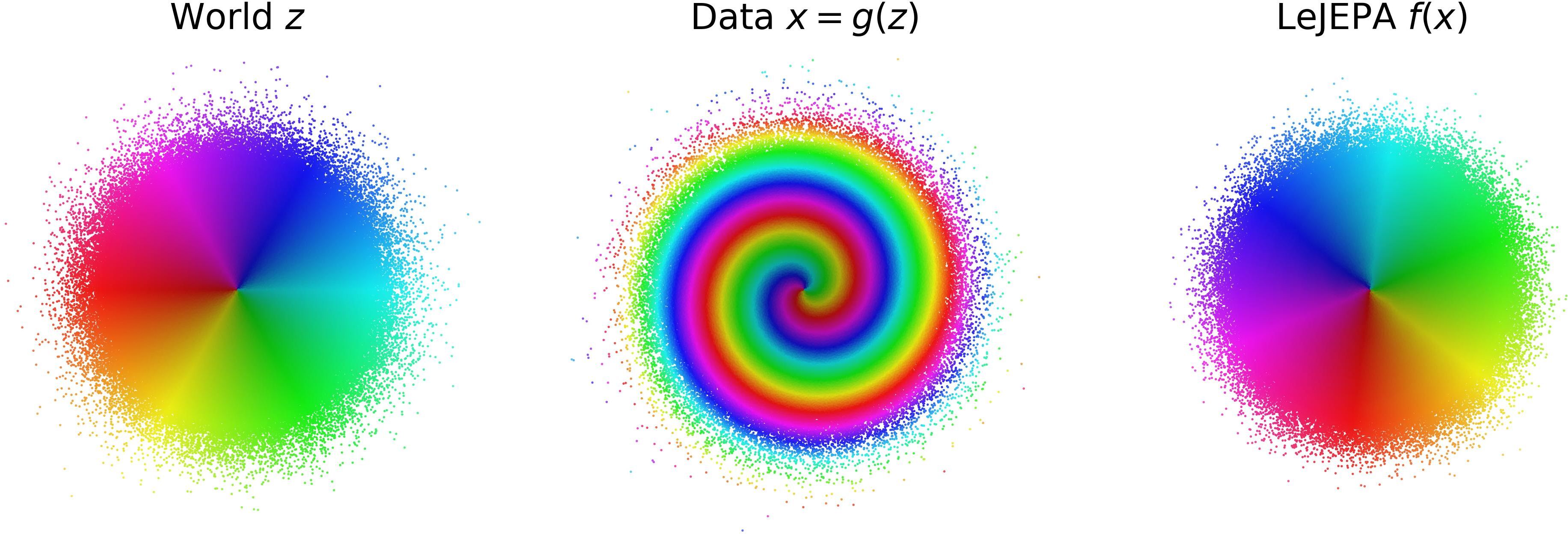
The paper proves that, in many cases, this forces the encoder to undo the camera’s warping and recover the hidden stats, up to a rotation. Rotation is fine because a round bell curve looks the same from any angle.

Key questions the paper answers

• When does LeJEPA recover the world’s hidden variables using only a simple linear (straight-line) formula?
• Is there something special about Gaussian (bell-curve) latent variables?
• What happens if the training isn’t perfect?
• Does recovering the hidden variables help us plan actions optimally?

How do they approach the problem?

The setup has two parts: the World and the Learner.

The World (data we observe)

• Hidden variables z (like positions or angles) follow a Gaussian (bell-curve) distribution.
• We never see z directly. An unknown nonlinear process g scrambles z into the observations x = g(z) we actually see (like a warped camera).
• We train on “positive pairs”: two related views of the same thing (for example, two close frames in time). Mathematically, the second view is a noisy, slightly changed version of the first. You can picture this as z’ being a slightly faded copy of z plus some random noise.

The Learner (LeJEPA)

• The encoder f maps observations x to embeddings y = f(x). Combined with g, this is a map h = f ∘ g that tries to “unscramble” the hidden variables.
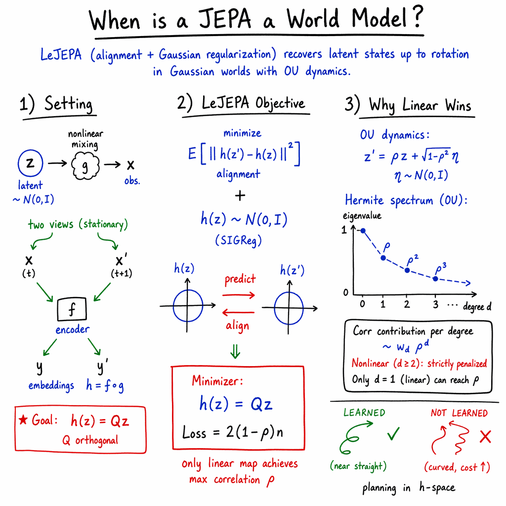
• Two goals: 1) Alignment: make h(z) and h(z’) close for positive pairs (pull related views together). 2) Gaussianity: make h(z) look like a round Gaussian (bell curve), to stop the representation collapsing and to keep it well-behaved.

Intuition: If every “wiggly” nonlinear part of h makes positive pairs less aligned, then the best h is a straight line. The Gaussianity rule then forces that straight line to be a rotation, which still preserves the bell curve shape.

Main results and why they matter

Below are the core findings, each explained simply.

LeJEPA recovers the hidden variables linearly

• Result: In a “Gaussian world” with the kind of positive pairs described above, any encoder that perfectly meets LeJEPA’s two goals must be linear and orthogonal: h(z) = Qz, where Q is a rotation/reflection.
• Why it matters: This means the representation isn’t mixing up unrelated factors (like position with color). It linearly recovers the true hidden stats, which is exactly what you want for simple downstream tasks and reliable planning.

The Gaussian is unique

• Result: Within this broad class of worlds (independent sources, stationary views, additive noise), the Gaussian distribution is the only one that guarantees this linear identifiability under LeJEPA.
• Why it matters: If the underlying hidden variables aren’t Gaussian, you can’t generally expect the learned representation to be linearly recoverable. This pinpoints when the method has a strong mathematical guarantee and when it doesn’t.

Approximate training still works well

• Result: If the model doesn’t perfectly meet the goals (which is normal in practice), the recovery error increases smoothly and predictably. There’s a simple bound showing how errors in alignment and Gaussianity affect how far h is from being a rotation of z.
• Why it matters: This gives confidence that near-perfect training still yields near-perfect recovery. It also tells practitioners that improving the alignment objective is especially important.

Planning in the learned space is optimal

• Result: If h is a rotation of the true hidden variables, then planning actions in the learned space is just as good as planning in the true hidden space, for a wide class of tasks whose costs don’t care about rotation (like “go straight to the goal”).
• Why it matters: This connects theory to action: a linearly identifiable representation isn’t just “nice”—it makes latent-space planning as good as planning with the true underlying state.

What experiments did they run?

The authors validate the theory with several experiments:

• Simple 2D worlds with different nonlinear scramblings: LeJEPA learns to “unscramble” them, recovering a round Gaussian up to rotation.
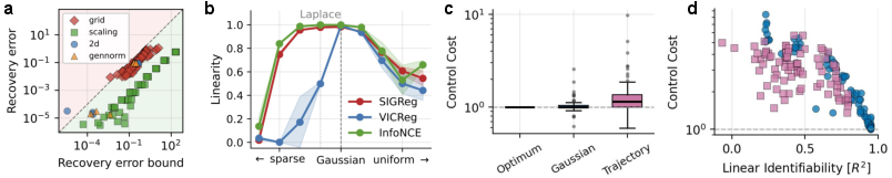
• Scaling to high dimensions (up to 1024): methods that enforce Gaussianity by batch statistics (like SIGReg and VICReg) keep excellent recovery as dimension grows.
• Non-Gaussian hidden variables: when the latent distribution isn’t Gaussian, recovery gets worse, matching the “Gaussian is unique” theorem.
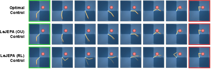
• Pixel-based robotic control: with real trajectories from a two-joint robot task, the data distribution is not Gaussian, and recovery is weaker; planning quality drops, just as predicted.
• Planning quality tracks identifiability: the closer the learned representation is to a rotation of the true state, the better the planned paths and control costs.

Why this is important

• Clarity: It turns a successful training recipe (LeJEPA) into a clear mathematical statement about when it truly learns the structure of the world.
• Reliability: Linearly identifiable representations are easier to use with simple tools (like linear probes) and are more robust when the world changes.
• Planning: If the representation is a rotation of the true state, we can plan in its space without losing optimality, which is crucial for robotics and control.

Implications and impact

• Data matters: If your training data explores the state space broadly and behaves like Gaussian latents with simple noisy transitions, LeJEPA gives strong guarantees.
• Objective design: Enforcing full Gaussianity in the embeddings (not just whitening) helps achieve the linear identifiability that makes planning reliable.
• Real-world systems: Many real systems aren’t perfectly Gaussian. The approximate bound helps in practice by showing performance degrades gracefully, and it highlights where better data collection or objective tuning can help.
• Foundation for World Models: These results provide a solid theoretical base for building learned models that reflect the true structure of the world, making them better for generalization, reasoning, and control.

Knowledge gaps, limitations, and open questions

Below is a concise list of concrete gaps and open questions that remain unresolved, focused on what is missing, uncertain, or left unexplored.

• Beyond Gaussian latents:
  • Does linear identifiability hold for non-Gaussian but structured latent families (e.g., elliptical Gaussians, mixtures of Gaussians, sub-Gaussian or heavy-tailed distributions) if the regularizer is adapted to the true latent distribution instead of enforcing isotropic Gaussianity?
  • Can LeJEPA be modified (e.g., with a distribution-matching regularizer learned from data) to achieve identifiability when $z$ is non-Gaussian?
• Independence and isotropy assumptions:
  • What happens when latent components are dependent (e.g., independent subspace analysis, correlated Gaussians, or weak dependencies)? Are there objective modifications that preserve linear identifiability under dependence?
  • The theory assumes a single, shared correlation $\rho$ across latent dimensions; what are the guarantees if correlations are anisotropic ($\rho_i$ vary by dimension) or time-varying?
• Transition model generality:
  • How do results change under more realistic transitions beyond stationary additive noise (e.g., multiplicative noise, non-Markovian dynamics, non-stationary processes, drift fields, or state-dependent diffusion)?
  • Can the spectral argument be extended to practical view-generating processes used in vision (e.g., crops, masking, color jitter), which are not additive-noise perturbations of latent variables?
• Observation process and realizability:
  • The theory reasons about $h = f \circ g$ on $z$ but does not require $g$ to be invertible; what minimal conditions on $g$ (e.g., injectivity, information-preservation) ensure that a realizable encoder $f(x)$ can achieve the optimal $h$?
  • How does observation noise in $x$ (sensor noise, compression artifacts) affect identifiability guarantees?
• Dimensionality mismatch and superposition:
  • When the encoder dimension $m \neq n$, which subspace is selected and under what conditions does superposition emerge or vanish? Can regularizers or architectural constraints guarantee unentangled selection of a correct $n$-dimensional subspace when $m > n$ and prevent loss of factors when $m < n$?
  • How can the true latent dimension be discovered rather than assumed?
• Approximate Gaussianity enforcement:
  • SIGReg is modeled as enforcing full Gaussianity, while the approximate theorem requires only near-whitening; what extra (practical) conditions on higher moments or distributional distance to Gaussian (e.g., Wasserstein, KL, or MMD) are sufficient for the Hermite-based argument to go through?
  • Can we bound identifiability as a function of deviation from Gaussianity beyond second-order moments (e.g., via cumulants or Hermite coefficients)?
• Finite-sample and optimization aspects:
  • What are sample-complexity rates for achieving small alignment gap $\delta$ and whitening error $\varepsilon$ as functions of $n$ and $\rho$, and how do these errors translate into end-to-end recovery error via tighter, dimension-aware constants?
  • How do training dynamics and optimization landscape affect convergence to the identifiable solution (local minima, implicit bias of SGD/architectures, batch-statistics noise)?
• Positive-pair design and ρ selection:
  • How should one design or learn positive-pair mechanisms to approximate the OU transition with a desirable $\rho$ in practice, especially from pixels? Can $\rho$ be estimated or controlled online to maximize identifiability?
  • When the real process yields anisotropic or highly concentrated marginals (as in policy-driven trajectories), what data-collection strategies or objective tweaks restore the conditions needed for identifiability?
• Planning guarantees and cost structure:
  • The planning equivalence requires $O(n)$-invariant costs. How do guarantees extend to non-rotation-invariant costs common in practice (e.g., joint-space penalties with different scales, obstacle costs), and what error bounds arise when this invariance is violated?
  • The planning theorem assumes access to the pushforward dynamics in the learned space; how do learned transition-model errors interact with the identifiability error to affect control performance?
• Generalization to sequences and multi-view setups:
  • Can leveraging multi-step or multi-view correlations (beyond single-step pairs) relax Gaussianity or independence assumptions and still yield linear identifiability?
  • How do results extend to hierarchical or multi-timescale latents (e.g., AR(p), switching dynamics, options)?
• Alternative alignment objectives:
  • The theory is stated for squared-distance alignment. Do analogous identifiability results hold for other JEPA objectives (e.g., cosine similarity, InfoNCE, Barlow Twins/VICReg variants) under comparable distributional constraints?
• Manifolds, periodicity, and discrete latents:
  • How do guarantees change for manifold-valued latents (e.g., tori for angles) or mixed discrete–continuous factors? Can LeJEPA be adapted to recover linearly identifiable embeddings of periodic or discrete variables?
• Robustness to heavy tails:
  • Empirically, identifiability degrades for heavy-tailed latents; what theoretical characterizations exist for the robustness of SIGReg or alternative regularizers under heavy-tailed distributions?
• Scope and external validity:
  • Empirical validation is limited (2D mixings, RealNVP, 1024-d latents, and one pixel-based robotics task). How does the theory fare on large-scale, natural video domains, diverse robotics settings, and other modalities (audio, multimodal)?
• Tightness and sharpening of the approximate bound:
  • The approximate bound depends on $\delta$ and $\varepsilon$ with coarse constants. Can it be tightened (e.g., dimension-adaptive constants, improved dependence on $\rho$), extended to account for higher-order deviations, and made robust to finite-sample estimators?
• Fairness and sensitivity in method comparisons:
  • Some InfoNCE results use fixed kernel width and degrade at scale; how sensitive are comparative conclusions to hyperparameter tuning (temperature, negatives, batch sizes) and estimator choices, and can theory explain such sensitivities?
• Toward action-conditioned identifiability:
  • The work acknowledges that action-conditioned transitions must be learned but does not provide identifiability guarantees in that setting. What assumptions on interventions/actions enable identifiability with LeJEPA-like objectives, and how do they connect to causal representation learning frameworks?

Immediate Applications

• Robotics (industrial, consumer, and research): Latent-space planning from pixels using LeJEPA-style encoders
  • What: Drop-in encoder training recipe (alignment + Gaussian regularization/SIGReg) that yields linearly identifiable latents, enabling straight-line planning in learned space to translate into optimal motion in the true system.
  • Where: Manipulation (arms, pick-and-place), mobile navigation, legged locomotion, home assistants, manufacturing cells.
  • How/tools:
  • Train encoders with LeJEPA (alignment + SIGReg) and high view-correlation (ρ close to 1) from video or simulated pixel streams.
  • Use the approximate bound to monitor identifiability during training: track covariance error ε and alignment gap δ; target low δ/(2ρ(1−ρ)).
  • Integrate a latent-space planner that uses O(n)-invariant costs (e.g., L2 goals, quadratic penalties) and Procrustes-aligned evals.
  • Value: Robust planning with fewer samples than pixel-space models; interpretable latent control; near-oracle performance on goal-reaching.
  • Assumptions/dependencies: Encoder output dimension matches latent dimension; costs are O(n)-invariant; positive pairs are highly correlated; data distribution not too far from Gaussian OU-like dynamics.
• Data collection strategy for self-supervised control pretraining
  • What: Replace goal-directed, narrow-coverage policies with isotropic, OU-like exploration to improve identifiability and downstream planning.
  • Where: Robotics labs, simulation farms, synthetic video generation pipelines.
  • How/tools:
  • “OU collector” environment wrapper that samples positive pairs with controlled ρ.
  • Replay buffer balancers to maintain marginal stationarity and coverage.
  • Value: Higher linear identifiability (R²⁾ and better planning quality compared to trajectories gathered under narrow, task-centric policies.
  • Assumptions/dependencies: Ability to control exploration policy; approximate stationarity; sufficient coverage of state space.
• Software engineering: Identifiability-aware JEPA training pipelines
  • What: Build training dashboards and checks that operationalize the theory as KPIs.
  • How/tools:
  • Metrics: ε = ||Cov(h(z))−I||F, δ = observed alignment loss − 2(1−ρ)tr(Cov(h(z))), identifiability error via orthogonal Procrustes, per-dimension correlations.
  • Alerts/early stopping: Use the bound D + (ε + D)² to stop, tune λ (regularization weight), and adjust ρ.
  • Prefer batch-statistic Gaussianity enforcers (SIGReg, VICReg) over InfoNCE at high dimensionalities; if using InfoNCE, tune kernel width with dimension.
  • Value: Predictable training outcomes; fewer failed runs; reproducibility and scale safety for large embeddings (up to ≥1024 dims demonstrated).
  • Assumptions/dependencies: Sufficient batch size for stable covariance estimates; correct loss implementation (e.g., SIGReg).
• Academic practice: Reproducible theory-to-empirics workflows and pedagogy
  • What:
  • Use released code and Lean-verified proofs to teach/replicate identifiability results.
  • Adopt linear probe evaluations as identifiability tests rather than generic proxy metrics.
  • Value: Clear benchmarks for when a representation is a “world model”; principled evaluation beyond task accuracy.
  • Assumptions/dependencies: Access to the provided repository; willingness to include identifiability diagnostics in standard SSL evaluations.
• Product design choices for SSL at scale (vision, video, robotics)
  • What: Prefer LeJEPA (alignment + Gaussianity) or VICReg over purely contrastive InfoNCE for large embedding dimensions; set λ small (less regularization weight) and ρ high to maximize linear recovery.
  • Value: Better scaling of identifiability and stability; simpler hyperparameter heuristics.
  • Assumptions/dependencies: Adequate compute and batch sizes; dataset provides correlated views (temporal neighbors or augmentations).
• Evaluation and auditing (“World Model Scorecards”)
  • What: Add identifiability scorecards to model audits, reporting R^2(h→z), ε, δ, and recovery error bounds.
  • Where: Industry model governance, academic benchmarks, internal research QA.
  • Value: Comparable, theory-grounded indicators that a model encodes a faithful world model rather than entangled or collapsed features.
  • Assumptions/dependencies: Access to synthetic “oracle latents” in controlled tests or strong proxies; standardized reporting templates.
• Sector-specific prototyping beyond robotics
  • Healthcare imaging: Pretrain encoders on OU-like sequential scans (e.g., respiratory cycles) to learn identifiable, denoised latents for downstream planning tasks (e.g., gated acquisition or beam steering).
  • Energy/smart grids: Identifiable latent states for short-horizon dispatch or load control where OU-like perturbations approximate stochastic fluctuations.
  • Finance/time series: Identifiability diagnostics for SSL embeddings; use in low-latency planning with near-Gaussian market microstructure segments.
  • Assumptions/dependencies: Approximate additive-noise stationarity; careful validation where independence across latent factors may be violated.

Long-Term Applications

• General-purpose world models with action-conditioned identifiability (causal control)
  • What: Extend identifiability guarantees to action-conditioned transitions p(z′|z,a), treating actions as interventions to recover causal latent structure.
  • Where: Robotics, autonomous driving, embodied AI.
  • Products/workflows: “Interventional LeJEPA” objectives; policy-aware data collection; action-latent disentanglement validators.
  • Dependencies: New theory for interventional identifiability; richer data with diverse actions; efficient exploration policies.
• Non-Gaussian worlds: Objective design for broader identifiability
  • What: Create regularizers and objectives that retain linear (or monotone) identifiability under non-Gaussian latent marginals observed in real trajectories.
  • Where: Real-world control, healthcare, econometrics.
  • Products: “Hermite lens” analyzers that quantify nonlinearity components; adaptive regularizers penalizing higher-order terms; SL-equation-guided losses.
  • Dependencies: Theory to characterize eigenfunctions under realistic noise and constraints; practical estimators for non-Gaussian score structure.
• Dimension-mismatch–resilient representations
  • What: Methods that preserve identifiability when embedding dim ≠ latent dim, mitigating superposition and redundancy.
  • Where: Foundation models with fixed-width embeddings, multimodal systems.
  • Products: Dimension selection/pruning utilities; structured sparsity or subspace selection during training; post-hoc disentanglement via spectral tools.
  • Dependencies: Theory bridging superposition with JEPA objectives; scalable estimators for intrinsic dimensionality online.
• Standardization and policy: Benchmarks and procurement criteria for “world models”
  • What: Establish identifiability-based standards for pretraining datasets, exploration regimes, and model evaluation in safety-critical systems.
  • Where: Robotics standards bodies, AV regulators, medical-device software compliance.
  • Products: Test suites with OU-like probes; reporting of ε, δ, and identifiability bounds; conformance certifications.
  • Dependencies: Community consensus; public benchmarks with reference implementations; sector-specific validation.
• Tooling for development lifecycle integration
  • What: IDE/ML-Ops plugins that continuously compute identifiability KPIs, surface recoverability warnings, and suggest data or hyperparameter fixes.
  • Where: ML platforms, internal research infra, cloud training services.
  • Products: “Identifiability Monitor” (dashboards, alerts, auto-tuning for λ and ρ); Procrustes-alignment probes in CI.
  • Dependencies: Efficient, low-overhead covariance and correlation estimators; scalable logging and evaluation pipelines.
• Education and workforce upskilling
  • What: Curricula and labs that connect JEPA training, spectral intuition (Hermite/SL), and control-theoretic planning equivalences.
  • Where: Universities, professional ML/robotics training, internal bootcamps.
  • Products: Lab packages using the open-source repo; Lean-proof walkthroughs; visualization tools for nonlinearity spectra.
  • Dependencies: Continued maintenance of open materials; community contributions.
• Cross-domain foundation models leveraging identifiability as a design constraint
  • What: Architectures that treat linear identifiability as a first-class objective alongside compression and transfer, to ease downstream control and reasoning.
  • Where: Vision-language-action systems, embodied multimodal agents, simulation-to-real transfer.
  • Products: “World Model Kit” combining LeJEPA encoders, OU-style data curation, and latent planners with O(n)-invariant costs.
  • Dependencies: Scalable data pipelines, multi-environment exploration, evaluation protocols spanning perception and control.

Notes on common assumptions and their impact on feasibility

• Gaussianity and OU-like transitions: Immediate gains when data can be collected or augmented to approximate stationary, additive-noise, Gaussian latents; otherwise, benefits taper (converse theorem).
• Independence across latent factors: Often violated in practice; approximate identifiability can still hold but may need tailored objectives or exploration.
• High pair correlation (ρ): Stronger guarantees and easier optimization; requires temporal adjacency or carefully designed positive pairs.
• Whitening/Gaussianization quality: Batch size and estimator stability affect ε; prefer batch-statistic approaches at scale.
• Cost design for planning: Benefits require O(n)-invariant stage/terminal costs; many quadratic or L2 goals already satisfy this.
• Training stability and monitoring: Use δ and ε as leading indicators; alignment is the primary bottleneck (dominant term in the bound).

• Additive noise: A perturbation model where independent noise is added to a signal or latent variable. "Additive noise. $z'_i = m_i(z_i) + \eta_i$ with $\eta_i$ independent of $z_i$."
• Alignment (loss): An objective that pulls embeddings of positive pairs closer together to enforce invariance. "Along with an alignment loss this enables stable end-to-end training from raw pixels"
• Approximate identifiability: A relaxed guarantee that the recovered latents are close (but not necessarily identical) to the true latents, degrading gracefully with objective errors. "We further prove an approximate identifiability result where the guarantee degrades gracefully,"
• Dirichlet energy: A functional measuring the smoothness (energy) of a mapping, often used in variational proofs. "We provide an alternative proof via Dirichlet energy and the Mazur--Ulam theorem in App.~\ref{app:dirichlet}, operating in a more theoretical ($\rho \to 1$) regime."
• Diffeomorphism: A smooth, invertible map with a smooth inverse. "These results typically constrain the representation to a smooth diffeomorphism;"
• Eigenfunction: A function that is mapped to a scaled version of itself by a linear operator. "a set of eigenfunctions $\varphi_k$ satisfying $T\varphi_k = \lambda_k \varphi_k$,"
• Eigenvalue: The scalar by which an eigenfunction is scaled under a linear operator. "with eigenvalues $$1 = \lambda_0 > \lambda_1 \geq \lambda_2 \geq \cdots \geq 0$$."
• Gaussianity regularizer: A regularization term that shapes the embedding distribution toward a Gaussian. "adds an explicit Gaussianity regularizer (SIGReg);"
• Hermite polynomials: An orthogonal polynomial basis natural for functions of Gaussian variables. "they are the Hermite polynomials $\{\mathrm{He}_k\}_{k \geq 0}$,"
• InfoNCE: A contrastive learning objective that uses negative samples to learn representations. "InfoNCE, VICReg, and LeJEPA span a hierarchy of Gaussianity constraints,"
• Isotropic Gaussian: A multivariate normal distribution with zero mean and identity covariance. "regularizing the embedding distribution toward an isotropic Gaussian via Sketched Isotropic Gaussian Regularization (SIGReg)."
• JEPA (Joint-Embedding Predictive Architectures): Architectures that predict in representation space by aligning embeddings of related views. "Joint-Embedding Predictive Architectures \citep[JEPAs,] []{lecun2022} pursue this vision"
• Latent-space planning: Planning actions directly in the learned latent representation rather than in observation space. "and show that linear, orthogonal identifiability enables optimal latent-space planning."
• LeJEPA: A JEPA variant combining alignment with Gaussian regularization to prevent collapse. "We prove that LeJEPA (alignment plus Gaussian regularization) linearly recovers the world's latent variables from nonlinear observations,"
• Linear identifiability: The property that the true latent variables can be recovered up to a linear transformation. "a property known as linear identifiability,"
• Mazur--Ulam theorem: A result stating that isometries between normed vector spaces are affine mappings. "We provide an alternative proof via Dirichlet energy and the Mazur--Ulam theorem in App.~\ref{app:dirichlet}"
• Mehler's formula: An identity relating Hermite polynomials and jointly Gaussian variables, used to derive eigenvalues by degree. "a consequence of Mehler's formula \citep{mehler1866}."
• Measure-preserving map: A transformation that preserves the underlying probability measure (distribution). "the spiral is measure-preserving, demonstrating that Gaussianity of the observations alone does not suffice for identifiability;"
• Nonlinear ICA: Independent Component Analysis with nonlinear mixing, typically unidentifiable without extra structure. "Nonlinear ICA is unidentifiable without additional structure \citep{hyvarinen1999,locatello2019}."
• Ornstein--Uhlenbeck (OU) transition: A Gaussian, mean-reverting Markov process that preserves Gaussian marginals under additive noise. "the Ornstein--Uhlenbeck (OU) transition \citep{uhlenbeck1930, doob1942}:"
• Orthogonal group O(n): The set of n×n orthogonal matrices (rotations/reflections) preserving Euclidean norms. "for some orthogonal $Q \in O(n)$."
• Pushforward: The distribution of a random variable after applying a measurable mapping. "Let $\hat p(\cdot \mid \hat z_t, a_t)$ denote the pushforward of $p$ under $h$,"
• RealNVP: A normalizing flow architecture using coupling layers for invertible transformations. "and a RealNVP-style coupling layer \citep{dinh2016density}."
• Score function: The derivative (gradient) of the log-density of a distribution. "Demanding an affine eigenfunction forces the score function $(\log p)'$ of the latent distribution to be linear."
• SIGReg (Sketched Isotropic Gaussian Regularization): A method that enforces Gaussian embeddings via sketch-based regularization to prevent collapse. "Sketched Isotropic Gaussian Regularization (SIGReg)."
• Slow Feature Analysis (SFA): A method that extracts features varying slowly over time or along transitions. "Most closely related is slow feature analysis (SFA) \citep{wiskott2002},"
• Spectral decomposition: Decomposing an operator into eigenfunctions/eigenvalues to analyze variance or predictability. "The forward direction rests on a spectral decomposition in which each degree of nonlinearity is strictly penalized by alignment,"
• Stationarity: The property that statistical distributions (e.g., marginals) remain constant across views or time. "Stationarity. Both views share the same marginal: $p(z) = p(z')$."
• Sturm--Liouville (SL) equation: A differential equation defining orthogonal eigenfunctions for certain operators, used to characterize transitions. "the eigenfunctions of the transition operator are characterized by a classical Sturm--Liouville (SL) equation \citep{sprekeler2014}."
• Transition operator: The operator mapping a function to its expected value at the next state under the world's dynamics. "define the transition operator $T$ by $(Th_i)(z) = \mathbb{E}[h_i(z') \mid z]$,"
• VICReg: A self-supervised objective enforcing invariance, variance, and covariance regularization without negatives. "covariance regularization \citep[VICReg,] []{bardes2022, zbontar2021},"
• Whitening: Transforming variables to have zero mean and identity covariance. "In addition, whitening (i.e., $\mathrm{Cov}(h(z)) = I_n$) fixes $$\mathbb{E}[\|h(z)\|^2] = \mathbb{E}[\|h(z')\|^2] = n$$,"
• World Model: An internal representation that captures the latent structure and dynamics of the environment. "When is a learned representation a World Model, i.e., a faithful map of the world's latent structure?"

Sign up for free to add this paper to one or more collections.